Other methods
During work for Robust uncertainty quantification…, we considered other methods. These were not included in the main text as they are retrospective rather than real-time (although they can be used for real-time analysis also). Preliminary results are included here.
We view this page as a living document. We have largely stuck to default options when implementing the various methods. If you think something can be improved, or you think something important is missing, please get in contact!
Executive summary
- We present and implement novel methods for evaluating existing models on observable data (calibration and CRPS of reported cases).
- EpiFilter (smoothing) generally performs the best, although this is partially due to matching assumptions about observation noise.
- The uniform/flat prior distribution used for EpiFilter’s smoothing parameter has a useful property: it ensures the MAP value is equal to the MLE. The predictive decomposition of the likelihood then ensures this is also the value that optimises one-step-ahead predictions. That is, using a flat prior distribution enforces a MAP that is optimal for one-step-ahead forecasting.
- EpiLPS(MALA) outperforms EpiLPS(MAP), most likely due to the proper handling of uncertainty in smoothing parameters. This supports our argument in Robust uncertainty quantification… that parameters should be marginalised out rather than fixed at some optimal value.
Background
Many state-of-the-art \(R_t\) estimation methods target the smoothing distribution, rather than the filtering distribution (see below). Examples include the smoothing version of EpiFilter (Parag 2021), EpiNow2 (Abbott et al. 2020), EpiLPS (Gressani et al. 2022), and rtestim (Liu et al. 2024). We compare and contrast these methods on simulated data here.
For each method, we:
- Find the posterior distribution for \(R_t\)
- Find the posterior “predictive” distribution for observed cases \(\tilde{C}_t\)
- Calculate the calibration of the implied 95% credible intervals for both \(R_t\) and \(C_t\)
- Calculate the CRPS of the posterior predictive distribution for \(C_t\)
We use \(\tilde{C}_t\) to highlight when we are treating reported cases as a random variable, instead of as observed data.
Unlike the other methods listed, rtestim is frequentist in nature. In this case, we replace posterior means/modes and credible intervals with estimates and confidence intervals. All of the above metrics still apply and carry comparable interpretations.
The posterior predictive distribution obtained from smoothing methods typically provides within-sample estimates. That is, the observed value \(C_t\) is used to find the posterior predictive distribution of \(\tilde{C}_t\). This can occur either indirectly (observed \(C_t\) informs \(R_t\) estimates, which then are used to predict \(\tilde{C}_t\)) or directly (observed \(C_t\) informs estimates of latent infection incidence, from which \(\tilde{C}_t\) are generated). This changes the interpretation of CRPS from a score of future predictions to a score of how well the data-generating mechanism is modelled.
In many cases, existing methodology had to be extended to find the posterior predictive distributions or to calculate the CRPS. Model descriptions are otherwise kept to a minimum. Where possible, default options of these models are used, although minor modifications are made where defaults lead to obviously suboptimal results.
Code to explicitly reproduce these results and figures is provided on GitHub.
Filtering versus smoothing
The filtering posterior distribution depends only on past data and is written \(P(R_t | C_{1:t})\), whereas the smoothing posterior distribution depends on all data and is written \(P(R_t | C_{1:T})\) (Särkkä 2013).
When producing estimates at the most recent time-step, only the filtering distribution is accessible, as future data are not yet available, whereas the smoothing distribution is generally preferred for retrospective analysis, as it incorporates all available data. Note that, at time \(t = T\), the filtering and smoothing distributions are equivalent.
In Robust uncertainty quantification in popular estimators of the instantaneous reproduction number, we focus on methods for estimating \(R_t\) in real-time. That is, we target the filtering distribution rather than the smoothing distribution1. Here we consider the latter.
Methods
EpiFilter (smoothing version)
In addition to the filtering distribution, EpiFilter also provides a method to find the smoothing distribution, conditional on smoothing parameter \(\eta\). Using the same arguments as for filtering, we marginalise over \(\eta\) to find the marginal smoothing distribution:
\[ P(R_t|C_{1:T}) = \int P(R_t | C_{1:T}, \eta) P(\eta | C_{1:T}) \ d\eta \]
This requires the posterior distribution for \(\eta\) once all data are collected: \(P(\eta|C_{1:T})\). We introduce methodology for this in Robust uncertainty quantification….
The posterior smoothing distribution for observed case incidence is found by marginalising over \(R_t\) from the smoothing posterior distribution for \(R_t\) (instead of the predictive distribution for \(R_t\)):
\[ P(\tilde{C}_t | C_{1:T}) = \int P(\tilde{C}_t | R_t, C_{1:T}) P(R_t | C_{1:T}) \ dR_t \]
For simplicity, we use the renewal model for \(P(\tilde{C}_t | R_t, C_{1:T})\), even though this ignores future reported case incidence. That is, future case data \(C_{t:T}\) only features in \(P(\tilde{C}_t | C_{1:T})\) via \(R_t\).
CRPS is calculated using the methodology outlined in Robust uncertainty quantification….
EpiNow2
Rather than using a Gaussian random walk (as in EpiFilter) or fixed sliding windows (as in EpiEstim), EpiNow2 models the evolution of \(R_t\) using a Gaussian process. The default implementation then assumes that latent infection incidence follows a deterministic renewal model. Reported cases are assumed to be negative binomially distributed around the true infection, with a day-of-the-week effect that is estimated during the fitting process. That is, EpiNow2 accounts for both process noise (in the evolution of \(R_t\)) and observation noise (in the distribution for reported cases).
Smoothness in \(R_t\) is primarily controlled by the Gaussian process kernel (default Matern 3/2, with lengthscale \(\ell\) and magnitude \(\alpha\)). In particular, prior assumptions about the lengthscale \(\ell\) have a significant impact on the smoothness of resulting estimates. It is also expected that prior assumptions about the observation overdispersion will have a secondary effect on the smoothness of \(R_t\) estimates (as this impacts the trade-off between process and observation noise).
The EpiNow2 package provides pre-built functionality to extract central estimates and credible intervals for \(R_t\) and observed cases. As far as we are aware, the package does not provide a method to calculate the CRPS, so we provide our own sample-based implementation.
Samples from the posterior distribution for reported cases \(\{x_t^{(i)}\}_{i=1}^N\) at time \(t\) are extracted from the Stan fit object. We then use the sample-based CRPS estimator:
\[ \text{CRPS}_t = \frac{1}{N} \sum_{i=1}^n |x_t^{(i)} - C_t| - \frac{1}{2N^2} \sum_{i=1}^n \sum_{j=1}^n |x_t^{(i)} - x_t^{(j)}| \]
Calculating this for each time-step \(t\) and taking the average gives the CRPS for observed case incidence. Code to reproduce this is available on GitHub.
By default, EpiNow2 uses a log normal prior distribution for the lengthscale \(\ell\) with mean 21 days and standard deviation 7 days. We also test an alternative and less informative inverse-gamma prior distribution provided with the package, which performs considerably better.
EpiLPS (MAP)
EpiLPS models latent infection incidence using Bayesian P-splines. Given infection incidence \(\mu(t)\) and overdispersion parameter \(\rho\), reported cases are assumed to be negative binomially distributed around \(\mu(t)\). In the maximum a posteriori (MAP) version of EpiLPS, central estimates of \(R_t\) are calculated using a plug-in estimate of the posterior mean incidence \(\hat{\mu}(t)\) and uncertainty is derived using a delta method. Like EpiNow2, EpiLPS explicitly accounts for both process noise (in the splines used to model infection incidence) and observation noise (in the distribution for reported cases).
Smoothness in \(R_t\) is primarily controlled by parameter \(\lambda\), where larger values penalise sharp changes in infection incidence. A hierarchical prior distribution is assumed for \(\lambda\). Prior assumptions about the overdispersion parameter \(\rho\) also likely impact the smoothness of \(R_t\) estimates, as this controls how much noise is associated with the observation process rather than the underlying epidemic process. The MAP version of EpiLPS selects optimal values of \(\lambda\) and \(\rho\) using an optimization routine.
While \(K = 30\) is used as the default number of splines, we find that this leads to inaccurate inference on our example datasets. For our examples, we increase this to \(K = 100\), which allows for more flexible inference.
We provide two extensions to the EpiLPS package:
- Methods to sample from the posterior distribution for reported cases.
- A CRPS estimator for the posterior distribution for reported cases.
Infection incidence is defined as \(\mu(t) = \exp(\theta^T b(t))\), where \(\theta\) is an estimated vector of spline coefficients and \(b(t)\) are the basis functions evaluated at time \(t\). The MAP version of EpiLPS uses a multivariate Gaussian approximation to \(\theta\) at the MAP estimate of \(\lambda\). We sample from this distribution:
\[ \theta^{(i)} \sim MVN(\hat{\theta}, Q_\lambda^{-1}) \]
and use these samples to generate samples of latent infection incidence:
\[ \mu^{(i)}(t) = \exp(\theta^{(i)T} b(t)) \]
from which samples of observed data are generated:
\[ C_t^{(i)} \sim \text{NegBin}(\mu^{(i)}(t), \rho) \]
where \(\rho\) is the MAP value of the overdispersion parameter. This is repeated \(N\) times (default \(N = 1000\)) at each value of \(t\). The mean of these \(N\) samples is reported as the central estimate, with 95% credible intervals obtained by taking the 2.5th and 97.5th percentile values.
The CRPS is calculated similarly, first by sampling \(\mu^{(i)}(t)\) as above and then using the crps_nbinom() function from the scoringRules package in R to calculate the CRPS value for each sampled \(\mu^{(i)}(t)\) and \(C_t\). The mean of these \(N\) CRPS values is reported as the CRPS for the \(t^{th}\) observed case incidence.
Some code is available on GitHub, although copyright limitations prevent us from providing the full implementation, in which case we outline the steps required to reproduce our analysis.
EpiLPS (MALA)
The MALA version of EpiLPS replaces the Laplace approximation and optimisation routine with a full MCMC-type sampler. This has the advantage of returning a posterior distribution on \(\lambda\) and \(\rho\), as well as properly marginalising out uncertainty about these quantities. As the true posterior distribution of spline coefficients \(\theta\) is targeted, we also expect the posterior distributions for \(R_t\) and observed cases incidence to be more accurate. This comes at a cost of slightly increased computational complexity, although we do not find this to be prohibitive.
The default version of EpiLPS(MALA) does not return the MCMC sampling object. In order to access this, we created a customised version of estimRmcmc.R that includes MCMC=MCMCout in the outputlist of the function. This is the sole change required to this script, although running it requires having local copies of some files from the EpiLPS package. A list of the required files is given here.
We make the same two extensions to EpiLPS(MALA) as we did to EpiLPS(MAP):
- Methods to sample from the posterior distribution for reported cases.
- A CRPS estimator for the posterior distribution for reported cases.
Samples of reported case incidence are extracted from the MCMC sampling object. For each sample \(i = 1, \ldots, N\) and time-step \(t = 1, \ldots, T\) we sample:
\[ C_t^{(i)} \sim \text{NegBin}(\exp(\theta^{(i)T} b(t)), \rho^{(i)}) \]
where \(\theta^{(i)}\) and \(\rho^{(i)}\) are samples from the MCMC sampling object. Note the use of \(\rho^{(i)}\) instead of the MAP value of \(\rho\), ensuring we are appropriately accounting for uncertainty in this parameter.
The CRPS is calculated from sampled \(C_t^{(i)}\) using the same approach as for EpiNow2, relying upon the sample-based CRPS estimator (see above).
Some code is available on GitHub, although copyright limitations prevent us from providing the full implementation, in which case we outline the steps required to reproduce our analysis.
rtestim
In contrast to the aforementioned Bayesian methods, rtestim is grounded in a frequentist framework. \(R_t\) is modelled using piecewise cubic functions with \(\ell_1\) regularisation on the divided differences. This regularisation enforces sparsity in changes in \(R_t\), allowing for locally adaptive smoothness, a key advantage over the other methods considered here that assume global smoothness.
A tuning parameter \(\lambda\) controls the strength of this regularisation, with larger values enforcing smoother estimates of \(R_t\). The optimal value of this parameter is automatically chosen by rtestim using cross-validation.
rtestim uses the delta method to calculate confidence intervals. Built-in functions are provided to calculate these for \(R_t\) and observed case incidence, for any user-specified significance level. To match the other methods we use a 95% confidence level.
While the frequentist framework of rtestim does not admit a posterior distribution for observed case incidence, we can still use CRPS to measure how well the confidence intervals approximate the observed distribution of the data. To do this, we treat the bounds of the confidence intervals at different significance levels as defining quantiles of an empirical CDF. That is, at each time-step \(t\), we find \(x_t^{(i)}\) such that \(q^{(i)} = F(x_i^{(t)})\) for \(q^{(i)} = 0.01, 0.02, \ldots, 0.99\). We then approximate the CRPS numerically at time-step \(t\) using the trapezoidal rule:
\[ CRPS_t = \sum_{i=1}^{n-1} \frac{1}{2} \left(x_t^{(i+1)} - x_t^{(i)}\right) \left[ \left(q^{(i+1)} - \mathbb{I}(x_t^{(i+1)} \geq y_t)\right)^2 + \left(q^{(i)} - \mathbb{I}(x_t^{(i)} \geq y_t)\right)^2 \right] \]
Averaging \(CRPS_t\) over all time-steps \(t\) gives the CRPS for observed case incidence. Code to reproduce this is available on GitHub.
Additional methodological notes
Each method handles the wind-in period differently, particularly when \(t\) is small compared to generation times. This can become fairly complicated, and is not the point of this supplementary section. When estimating or calculating coverage and CRPS, we use time-steps \(t = 10, \ldots, T\) to avoid differences from this period impacting our results.
Posterior parameter values were calculated using a grid-based approach for EpiFilter. For EpiLPS (MALA) and EpiNow2, a sampling approach was required. The mean, 2.5th and 97.5th quantiles of these samples were calculated to estimate the posterior mean and 95% credible intervals. Posterior mode values were calculated using a kernel density estimate from the default density() function in R.
Results
Theoretical links between Gaussian random walks, Gaussian processes, splines, and piecewise polynomials, as well as the fact that all models use the same underlying renewal model for the epidemic process, suggest that the methods should perform similarly in practice. However, we find this not to be the case.
Table 1 presents the coverage of \(R_t\) and reported cases, as well as the CRPS for reported cases for each method on each of the three simulations considered in the main text. Figure 1 presents the corresponding estimates. While the methods produce mostly well-calibrated 95% uncertainty intervals for observed case data, coverage of \(R_t\) estimates varies significantly, as does the CRPS for observed case incidence.
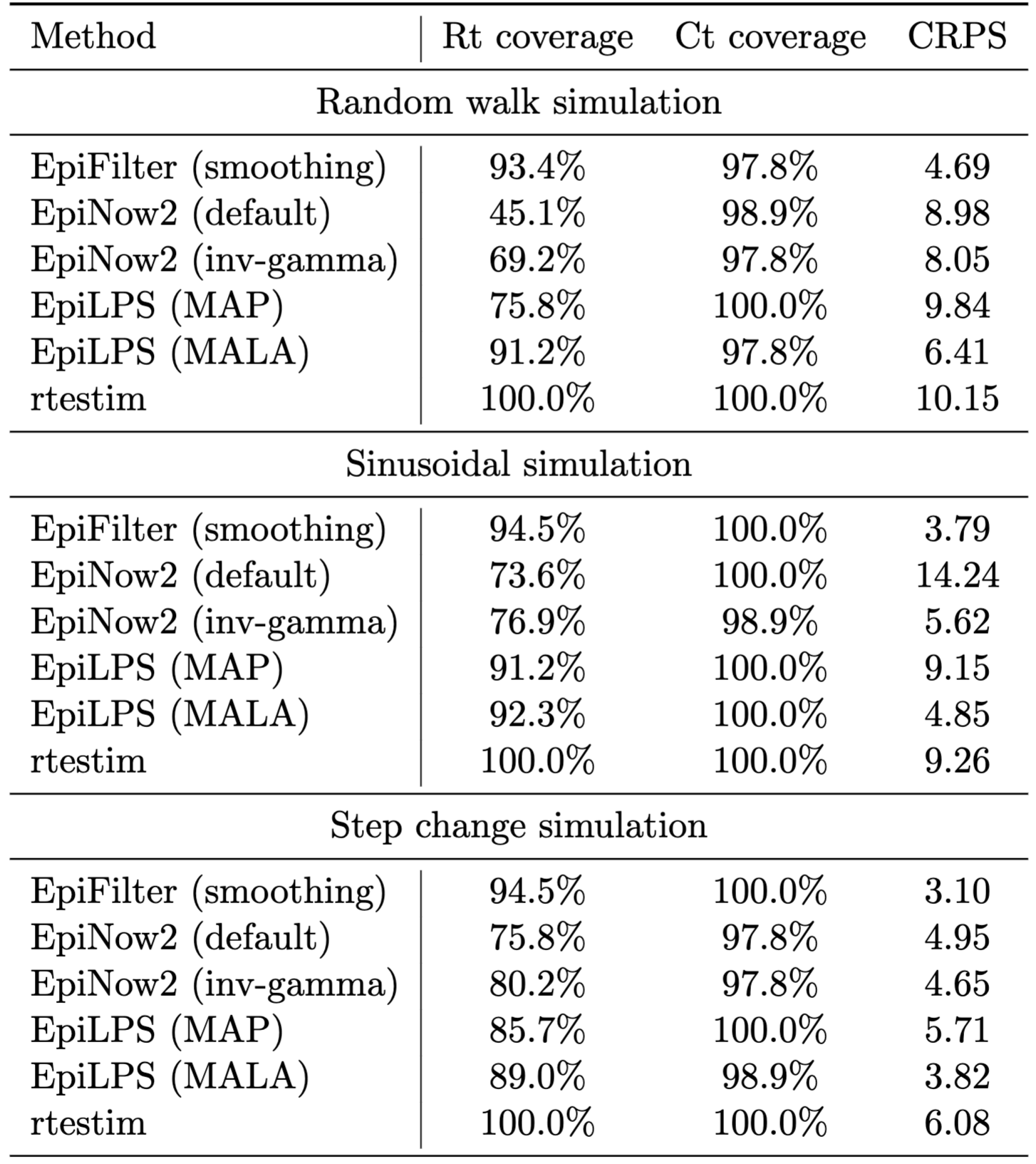
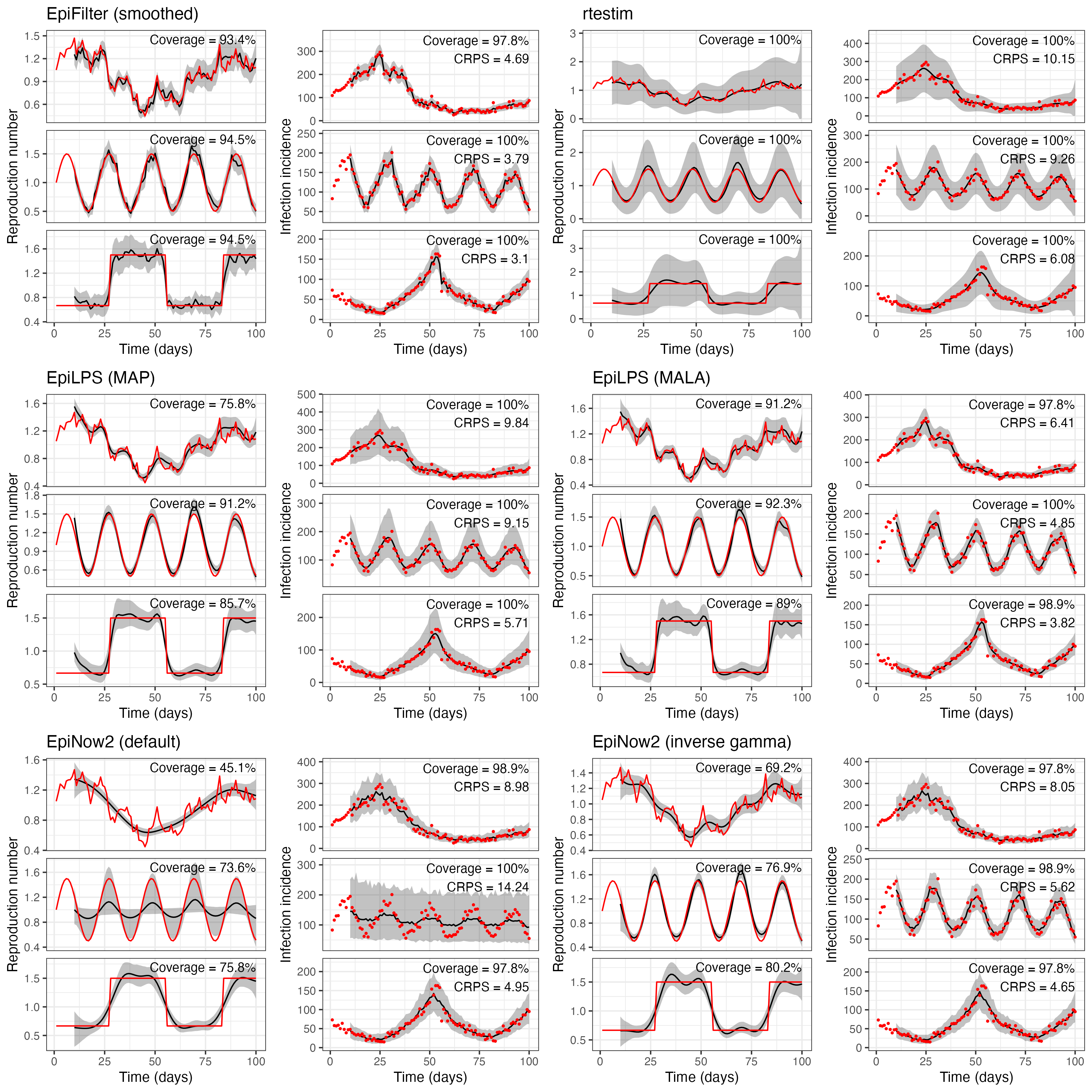
The smoothed version of EpiFilter consistently outperforms (i.e. exhibits coverage of 95% credible intervals closest to 95%, and the lowest CRPS values) the other methods on these simulated datasets. This is expected in the random walk simulation, where the dynamic model employed by EpiFilter matches the simulated data. The better performance of EpiFilter on the other simulations is likely explained by two factors: (1) EpiFilter does not account for observation noise (which is absent in the simulated data), and (2) the flat prior distribution on \(\eta\) is less informative than the default prior distributions used by other methods. These are both testable hypotheses that could be explored in future work to better understand the trade-offs between smoothing, model assumptions, and robustness of performance.
EpiLPS and EpiNow2 both assume that reported case incidence are negative binomially-distributed about some smooth true infection incidence (upon which the renewal model is placed), thus explicitly modelling observation noise. Process noise is derived from either the smoothness of the splines (EpiLPS) or the Gaussian process (EpiNow2). While the overdispersion parameter is estimated in both methods, the negative binomial distribution implies a lower bound of Poisson observation noise. In the simulated data, however, all noise is assumed to arise from the underlying process. By enforcing the inclusion of observation noise, EpiLPS and EpiNow2 underestimate process noise, and thus produce overly smooth estimates of \(R_t\). This is likely to be less impactful on real-world datasets, where observation noise is typically a significant factor.
It is possible to use CRPS as model selection criterion instead of cross-validation. Early code to do this is provided on GitHub.
The MALA version of EpiLPS outperforms the MAP version. This is unsurprising given that, in the MALA version, uncertainty associated with \(\lambda\) and \(\rho\) is fully marginalised out, whereas the MAP version selects optimal point estimates of these parameters. This lends support to the argument in the main paper for the marginalisation of these parameters over selection. The MALA version also targets the true posterior distribution for \(\mu(t)\), whereas the MAP version uses a Laplace approximation, which is particularly advantageous when comparing CRPS values.
Figure 1 also highlights critical oversmoothing in default EpiNow2 on the sinusoidal simulation. The posterior distribution for lengthscale \(\ell\) is bi-modal, with one mode at a small value of \(\ell\) (where the model follows the data) and another mode at a larger value of \(\ell\), where the model estimates flat incidence with large reporting noise accounting for changes in observed cases.
Prior distributions on smoothing parameters
While all methods listed estimate smoothing parameter(s) from the data, they handle this in different ways. Our implementation of EpiFilter, EpiNow2, and EpiLPS(MALA) marginalise this parameter out. EpiLPS(MAP) and rtestim select optimal point values of this parameter.
Of particular note is EpiNow2’s prior on lengthscale \(\ell\). Prior and posterior modes and credible intervals are give in Table 2. The default log-normal prior distribution often leads to oversmoothing, with an extreme example being the bimodal posterior on the sinusoidal simulation - where one mode implies that \(R_t\) is (nearly) fixed, and all variation in reported cases is assigned to the observation process.
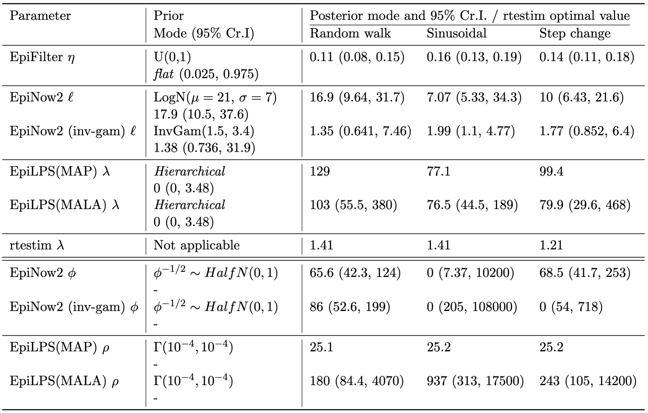
By default, we place a uniform prior distribution on EpiFilter’s \(\eta\) parameter. While we avoid claiming that the uniform prior distribution is uninformative, we do highlight a key advantage of this: the MAP is equal to the MLE. By the predictive decomposition of the likelihood, this is also the value of \(\eta\) that optimises one-step-ahead predictions. That is, using a flat prior distribution enforces a MAP that is optimal for one-step-ahead forecasting. Furthermore, if the model is correctly specified, this implies that the MAP is optimal for any n-step-ahead forecast.
References
Footnotes
The “smoothing” in “smoothing distribution” has a different meaning to “smoothing” in “smoothing parameter”.↩︎