Sequential Monte Carlo (SMC) methods are a class of methods used to solve hidden-state models.
It is helpful to define some general notation:
- \(X_t\) - hidden-states (such as the reproduction number \(R_t\) or infection incidence \(I_t\))
- \(y_t\) - observed data (such as reported cases \(C_t\))
- \(\theta\) - model parameters that don’t change over time
Depending on your goal, you may only care about some of these terms, and might want to marginalise out the terms you’re not interested in. Nevertheless, it is important to consider all three.
If your goal is forecasting, then future observed data \(Y_{t+k}\) are your quantity of interest, and you only care about \(X_t\) and \(\theta\) to the extent that they allow you to estimate \(Y_{t+k}\).
If your goal is reproduction number estimation (or the estimation of any hidden-state), then \(\theta\) is often a nuisance parameter which you only care about to the extent that it allows you to estimate \(R_t\).
If your goal is to learn about \(\theta\), which may represent the effect of a non-pharmaceutical intervention, for example, then \(\theta\) is likely your quantity of interest, and you only care about \(X_t\) to the extent that it allows you to estimate this effect.
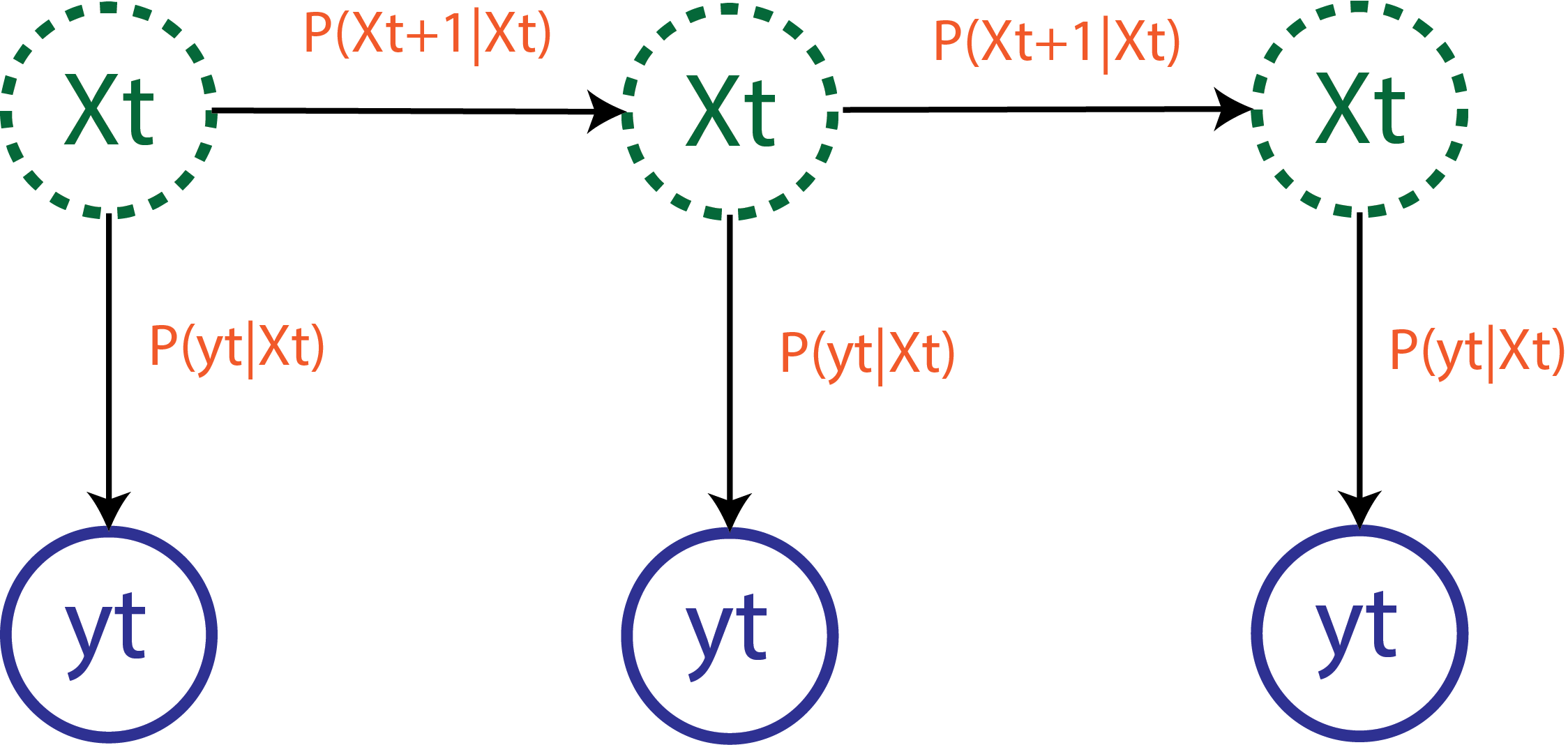
Definition: hidden-state model
A hidden-state model has two components:
A state-space transition distribution:
\[
P(X_t | X_{1:t-1}, \theta)
\tag{3.1}\]
which dictates how the hidden-states vary over time.
An observation distribution: \[
P(y_t | X_{1:t-1}, y_{1:t-1}, \theta)
\tag{3.2}\]
which relates the observed data to the hidden-states.
These two distributions wholly define the model.
This structure makes it clear why hidden-state models are so popular in epidemiology. The underlying epidemic is often unobserved (thus represented by the state-space model), while reported cases (or other data) are generated through some observation process.
We note that we make no Markov-type assumption, although Markovian models (a.k.a. Hidden Markov Models (Kantas et al. 2015) or POMPs (King, Nguyen, and Ionides 2016)) can be viewed as a special case of these hidden-state models.
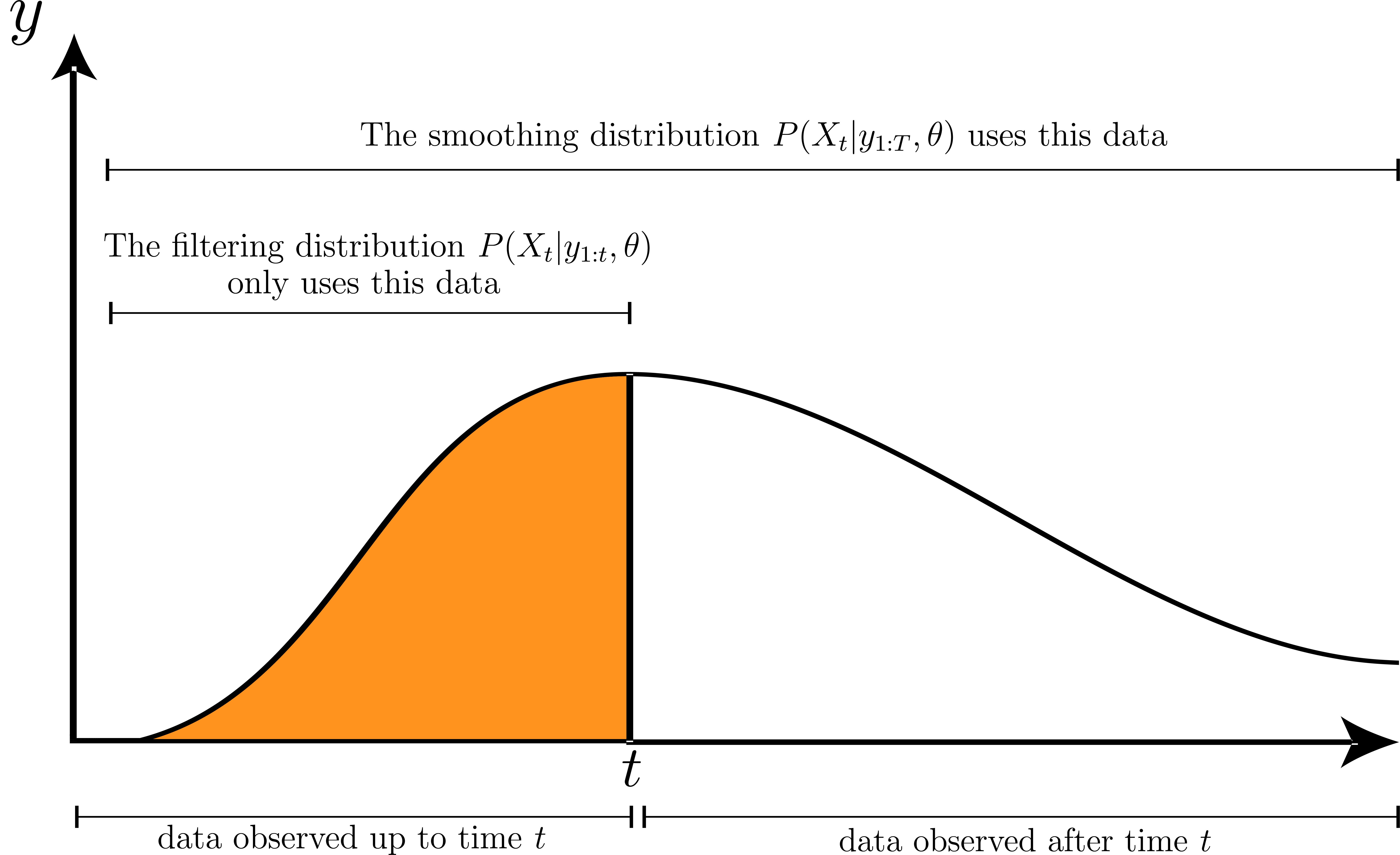
Filtering and smoothing distributions
Borrowing language from signal processing, we highlight two different posterior distributions for \(R_t\) that we may be interested in (Särkkä 2013).
The conditional filtering distribution is defined as:
\[
P(X_t | y_{1:t}, \theta)
\tag{3.3}\]
while the conditional smoothing distribution is defined as:
\[
P(X_t | y_{1:T}, \theta)
\tag{3.4}\]
The filtering distribution uses only past observations to estimate the hidden-states, whereas the smoothing distribution uses both past and future observations.
One of the strengths of EpiFilter (Parag 2021) is its ability to find the smoothing distribution, allowing more data to inform \(R_t\) estimates, particularly improving inference in low-incidence scenarios.
We demonstrate SMC methods suitable for finding both distributions.
Examples
We present three examples of increasing complexity. While all examples are relatively simple, many off-the-shelf methods are unable to fit the third example model.
Example 1: a simple model
In Section 1.2 we introduced a simple model for \(R_t\) estimation. We can write this model in the form of a hidden-state model.
The Gamma\((a_0, b_0)\) prior distribution on \(R_t\) forms the state-space transition distribution:
\[
R_t \sim \text{Gamma}(a_0, b_0)
\tag{3.5}\]
while the Poisson renewal model with mean \(R_t \Lambda_t\) forms the observation distribution:
\[
C_t | R_t, C_{1:t-1} \sim \text{Poisson}(R_t \Lambda_t^c)
\tag{3.6}\]
The sole time-varying hidden-state is the reproduction number \(R_t\), the observed data are reported cases \(C_{1:T}\), and the model parameters are \(a_0\), \(b_0\), and \(\{\omega_u\}_{u=1}^{u_{max}}\). Altogether this forms our hidden-state model.
We previously solved this hidden-state model in Section 1.2 by leveraging the conjugacy of the state-space model with the observation model. Such conjugacy is rare, hence state-space models are often solved using SMC (or other simulation-based methods).
Side-note: the state-space transition distribution for \(R_t\) does not depend on previous values of \(R_t\), so calling it a “transition” distribution might feel strange. Nevertheless, the model still fits in this framework!
Example 2: EpiFilter
EpiFilter (Parag 2021) is an example of a typical state-space model. Autocorrelation in \(R_t\) is modelled using a Gaussian random walk, defining the state-space model as:
\[
R_t | R_{t-1} \sim \text{Normal}\left(R_{t-1}, \eta \sqrt{R_{t-1}}\right)
\tag{3.7}\]
with initial condition \(R_0 \sim P(R_0)\). The gaussian random walk acts to smooth \(R_t\) (see Section 1.2.2). Like Example 1 above, EpiFilter also uses the Poisson renewal model as the observation distribution:
\[
C_t | R_t, C_{1:t-1} \sim \text{Poisson}(R_t \Lambda_t^c)
\tag{3.8}\]
As before, the hidden-states are the collection of \(R_t\) values, and the observed data are reported cases \(C_{1:T}\). Model parameters are now \(\eta\) (which controls the smoothness of \(R_t\)), \(\{\omega_u\}_{u=1}^{u_{max}}\), and \(P(R_0)\).
No analytical solution to the posterior distribution for \(R_t\) exists, however Parag (2021) avoid the need for simulation-based methods through the use of grid-based approximations.
Example 3: Modelling infection incidence
In Section 1.4 we highlighted that the renewal model can be placed on either reported cases (as in the examples so far) or “true” infection incidence. Let’s now assume that reported cases are observed with Gaussian noise about the true number of infections.
We keep the same state-space model for \(R_t\), and now assume that infection incidence \(I_t\) (also a hidden-state) follows the renewal model, resulting in the following state-space model: \[
R_t | R_{t-1} \sim \text{Normal}\left(R_{t-1}, \eta \sqrt{R_{t-1}}\right)
\]
\[
I_t | R_t, I_{1:t-1} \sim \text{Poisson}(R_t \Lambda_t)
\]
With our observation distribution now taking the form:
\[
C_t \sim \text{Normal}(I_t, \phi)
\]
While appearing simple, there are a number of reasons why existing methodology stuggles to fit this model. The new state-space model is non-Markovian, thus the grid-based approach used by EpiFilter (and many other methods developed for hidden Markov models) no longer works. Furthermore, \(I_t\) is integer-valued so the model cannot be fit using popular probabilistic programming languages like Stan.
Kantas, Nikolas, Arnaud Doucet, Sumeetpal S. Singh, Jan Maciejowski, and Nicolas Chopin. 2015.
“On Particle Methods for Parameter Estimation in State-Space Models.” Statistical Science 30 (3): 328–51.
https://doi.org/10.1214/14-STS511.
King, Aaron A., Dao Nguyen, and Edward L. Ionides. 2016.
“Statistical Inference for Partially Observed Markov Processes via the R Package Pomp.” Journal of Statistical Software 69 (12).
https://doi.org/10.18637/jss.v069.i12.
Parag, Kris V. 2021.
“Improved Estimation of Time-Varying Reproduction Numbers at Low Case Incidence and Between Epidemic Waves.” PLOS Computational Biology 17 (9): e1009347.
https://doi.org/10.1371/journal.pcbi.1009347.
Särkkä, Simo. 2013.
Bayesian Filtering and Smoothing. 1st ed. Cambridge University Press.
https://doi.org/10.1017/CBO9781139344203.