1  The renewal model

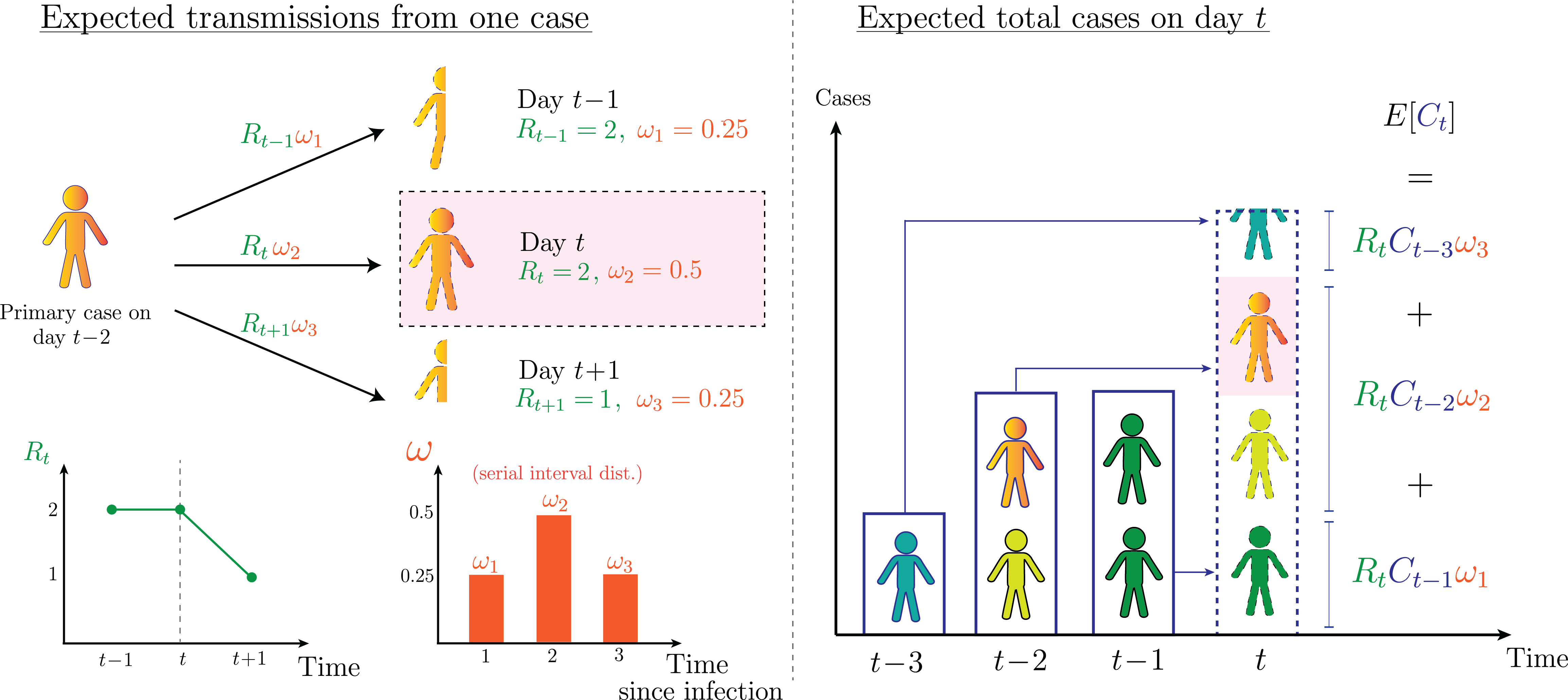
The renewal model is a simple model of infectious disease transmission. It relates past cases to current cases through a serial interval and reproduction number. It is typically written:

\[ E[C_t] = R_t \sum_{u=1}^{u_{max}} C_{t-u} \omega_u \tag{1.1}\]

where:

• \(C_t\): the number of cases reported on time-step \(t\)
• \(R_t\): the instantaneous reproduction number at time-step \(t\). Defined as the average number of secondary cases produced by an infected individual, if they were to have their entire infectious period at the current time-step.
• \(\omega_u\): the serial interval. The probability that a secondary case was reported \(u\) days after the primary case. \(u_{max}\) denotes the maximum value of \(u\) for which \(\omega_u > 0\).

Figure 1.1: Simple diagram outlining the renewal equation

We also need to specify a distribution for \(C_t\). The canonical choice is the Poisson renewal model:

\[ C_t|R_t, C_{1:t-1} \sim \text{Poisson}\left(R_t \sum_{u=1}^{u_{max}} C_{t-u} \omega_u \right) \tag{1.2}\]

Finally, we often denote the summation in the renewal model using:

\[ \Lambda_t^c = \sum_{u=1}^{u_{max}} C_{t-u} \omega_u \tag{1.3}\]

where \(\Lambda_t^c\) is called the force-of-infection at time \(t\). The superscript \(c\) denotes that \(\Lambda_t^c\) is calculated using past reported cases, to differentiate it from \(\Lambda_t\), which we use when modelling infections.

1.1 Simulating the renewal model

To understand how the renewal model works, let’s start by simulating \(T = 100\) days of reported cases from it. To do this, we need three components:

1. Initial cases \(C_1\). Let’s start with \(C_1 = 50\).

T = 100
C = zeros(T) 
C[1] = 50 

2. The reproduction number over time. We will use a sin-curve for this example:

R = 1.0 .+ 0.5 * sin.((2*π/50) .* (1:T))

3. A serial interval. We use a discretised Gamma(2.36, 2.74)¹ distribution:

using Distributions

ω = pdf.(Gamma(2.36, 2.74), 1:T)
ω = ω/sum(ω) # Ensure it is normalised!

Plotting our chosen \(R_t\) and serial interval:

# Visualise Rt and the serial interval
using Plots, Measures
plotR = plot(R, label=false, xlabel="Time (days)", ylabel="Reproduction number", color=:darkgreen)
plotω = bar(1:21, ω[1:21], label=false, xlabel="Day", ylabel="Serial interval probability", color=:darkorange)
display(plot(plotR, plotω, layout=(1,2), size=(800,300), margins=3mm))

Figure 1.2: Assumed time-varying reproduction number and serial intervals.

Now we are ready to simulate from the renewal model. We do this by iteratively sampling a new \(C_t\) and calculating the new force-of-infection term:

for tt = 2:T

    # Calculate the force-of-infection
    Λ = sum(C[tt-1:-1:1] .* ω[1:tt-1])/sum(ω[1:tt-1])

    # And sample from the appropriate Poisson distribution
    C[tt] = rand(Poisson(R[tt] * Λ))

end

Finally letting us plot our simulated cases:

display(bar(C, label=false, xlabel="Time (days)", ylabel="Simulated cases", size=(800,300), margins=3mm, color=:darkblue))

Figure 1.3: Simulated epidemic from the renewal model using our chosen values of Rt and ω.

1.2 Estimating \(R_t\)

\(R_t\) is a crucial component in the renewal model thus making the renewal model a natural choice for \(R_t\) estimation. In fact, even if your goal is not to estimate \(R_t\), it is helpful to consider this briefly.

If \(C_t\) is large and the model accurately reflects reality, we can use Equation 1.2 to estimate \(R_t\) directly. In the Bayesian setting, a prior distribution is placed on \(R_t\) and standard methods are used to find \(P(R_t | C_{1:t})\). However, often \(C_t\) is small and the data are subject to noise and bias. Estimates from the naive method are thus highly variable.

1.2.1 Example

Let’s pretend we don’t know \(R_t\) and want to estimate it from the simulated data. Like Cori et al. (2013), we will use a Gamma prior distribution for \(R_t\) with shape \(a_0 = 1\) and rate \(b_0 = 0.2\). As our likelihood is a Poisson distribution, we have a conjugate prior-likelihood, and thus our posterior distribution for \(R_t\) is:

\[ R_t | C_{1:t} \sim \text{Gamma}\left(a_0 + C_t, b_0 + \sum_{u=1}^{u_{max}} C_{t-u} \omega_u \right) \tag{1.4}\]

(MeanRt, LowerRt, UpperRt) = (zeros(T), zeros(T), zeros(T)) # Pre-allocate results vectors
(a0, b0) = (1, 1/5) # Set prior parameters

for tt = 2:T

    # Find the posterior distribution on day t
    a = a0 + C[tt]
    b = b0 + sum(C[tt-1:-1:1] .* ω[1:tt-1])/sum(ω[1:tt-1])
    PosteriorDist = Gamma(a, 1/b)

    # Save the results
    MeanRt[tt] = mean(PosteriorDist)
    LowerRt[tt] = quantile(PosteriorDist, 0.025)
    UpperRt[tt] = quantile(PosteriorDist, 0.975)

end

We will compare our estimates with those from a popular model, EpiEstim, which smooths the data by assuming \(R_t\) is fixed over a \(\tau\)-day (typically \(\tau = 7\)) trailing window:

include("../src/RtEstimators.jl")
EpiEstimPosterior = EpiEstim(7, ω, C; a0=a0, b0=b0)
(EpiEstMean, EpiEstLower, EpiEstUpper) = (mean.(EpiEstimPosterior), quantile.(EpiEstimPosterior, 0.025), quantile.(EpiEstimPosterior, 0.975))

Finally, we are ready to plot our results:

plot(xlabel="Time (days)", ylabel="Reproduction number", size=(800,350), left_margin=3mm, bottom_margin=3mm)
plot!(2:T, MeanRt[2:T], ribbon=(MeanRt[2:T]-LowerRt[2:T], UpperRt[2:T]-MeanRt[2:T]), fillalpha=0.4, label="Unsmoothed posterior")
plot!(2:T, EpiEstMean[2:T], ribbon=(EpiEstMean[2:T]-EpiEstLower[2:T], EpiEstUpper[2:T]-EpiEstMean[2:T]), fillalpha=0.4, label="EpiEstim (smoothed) posterior")
plot!(1:T, R, label="True Rt", color=:black)

Figure 1.4: Estimates of Rt from the basic (unsmoothed) renewal model (blue) and from a smoothed model (EpiEstim, orange).

1.2.2 The necessity and dangers of smoothing

?fig-intro-exampleRt highlights both the necessity and dangers of smoothing. Our independent daily estimates (blue) are highly variable and the credible intervals are wide. By using smoothed estimates (orange), we reduce this variance and produce much more confident results. However, our results strongly depend on these smoothing assumptions. In the example above, we can clearly see that the credible intervals produced by EpiEstim often do not include the true value of \(R_t\)!

Smoothing works by allowing data from multiple days to inform point-estimates. A variety of approaches have been developed, discussed at length in Appendix C. In fact, most renewal-model based estimators of \(R_t\) differ only in their choice of smoothing method!

Epidemic renewal models are usually smoothed by placing assumptions on the dynamics of \(R_t\). Examples include assuming \(R_t\) is fixed over trailing windows (Cori et al. 2013), modelling it with splines (Azmon, Faes, and Hens 2014) or Gaussian processes (Abbott et al. 2020), or assuming it follows a random walk (Parag 2021). Piecewise-constant models, where \(R_t\) is assumed to be fixed over different time-windows, are also examples of smoothing (Creswell et al. 2023).

So far we have only considered process noise in the epidemic, but epidemic data are often subject to observation noise, a secondary reason why smoothing is so important. We elaborate on this in #TODO.

1.3 The serial interval

The other key component in the renewal model is the serial interval \(\omega\). This parameter is typically not identifiable from reported case data (at least at the same time as \(R_t\)), so it often receives less attention. When fitting renewal models, researchers usually use estimates of the serial interval from other data.

External estimates of \(\omega\).

1.4 Reported cases vs infections

The simple renewal model in Equation 1.2 assumes that old reported cases directly cause new reported cases. This leaves little room for observation noise. Instead, we can assume that old (but typically unobserved) infections cause new infections, writing:

\[ I_t|R_t, I_{1:t-1} \sim \text{Poisson}\left(R_t \Lambda_t\right) \tag{1.5}\]

The force-of-infection becomes:

\[ \Lambda_t = \sum_{u=1}^{u_{max}} I_{t-u} g_u \tag{1.6}\]

Where we have replaced the serial interval \(\omega_u\) with a generation time distribution \(g_u\), reflecting that we are modelling the delay between infection events instead of reporting events.

Explicitly modelling infections allows us to define an observation distribution:

\[ P(C_t | I_{1:t}) \tag{1.7}\]

which explicitly links our hidden (a.k.a latent) infections to our reported cases. A plethora of methods exist that can estimate \(I_{1:T}\) given \(C_{1:T}\).

Separating case reporting from transmission allows us to model process noise and observation noise separately. This is one of the key advantages provided by our SMC methods.

Abbott, Sam, Joel Hellewell, Robin N. Thompson, Katharine Sherratt, Hamish P. Gibbs, Nikos I. Bosse, James D. Munday, et al. 2020. “Estimating the Time-Varying Reproduction Number of SARS-CoV-2 Using National and Subnational Case Counts.” Wellcome Open Research 5 (December): 112. https://doi.org/10.12688/wellcomeopenres.16006.2.

Azmon, Amin, Christel Faes, and Niel Hens. 2014. “On the Estimation of the Reproduction Number Based on Misreported Epidemic Data.” Statistics in Medicine 33 (7): 1176–92. https://doi.org/10.1002/sim.6015.

Cori, Anne, Neil M. Ferguson, Christophe Fraser, and Simon Cauchemez. 2013. “A New Framework and Software to Estimate Time-Varying Reproduction Numbers During Epidemics.” American Journal of Epidemiology 178 (9): 1505–12. https://doi.org/10.1093/aje/kwt133.

Creswell, Richard, Martin Robinson, David Gavaghan, Kris V. Parag, Chon Lok Lei, and Ben Lambert. 2023. “A Bayesian Nonparametric Method for Detecting Rapid Changes in Disease Transmission.” Journal of Theoretical Biology 558 (February): 111351. https://doi.org/10.1016/j.jtbi.2022.111351.

Ferguson, N, D Laydon, G Nedjati Gilani, N Imai, K Ainslie, M Baguelin, S Bhatia, et al. 2020. “Report 9: Impact of Non-Pharmaceutical Interventions (NPIs) to Reduce COVID19 Mortality and Healthcare Demand.” Imperial College London. https://doi.org/10.25561/77482.

Parag, Kris V. 2021. “Improved Estimation of Time-Varying Reproduction Numbers at Low Case Incidence and Between Epidemic Waves.” PLOS Computational Biology 17 (9): e1009347. https://doi.org/10.1371/journal.pcbi.1009347.

Parag, Kris V., Benjamin J. Cowling, and Christl A. Donnelly. 2021. “Deciphering Early-Warning Signals of SARS-CoV-2 Elimination and Resurgence from Limited Data at Multiple Scales.” Journal of The Royal Society Interface 18 (185): 20210569. https://doi.org/10.1098/rsif.2021.0569.

---

1. This is a popular serial interval used in early COVID-19 models (Parag, Cowling, and Donnelly 2021; Ferguson et al. 2020).