This chapter assumes fixed and known values of the model parameters. Chapter 5 considers the estimation of \(\theta\).
4.1 Background
Goal
The goal of the bootstrap filter is to use observed data \(y_{1:T}\) to learn about the hidden-states \(X_t\) given a pre-determined parameter vector \(\theta\).
The fundamental idea of the bootstrap filter (and particle filters in general) is to produce collections of samples from the target posterior distribution of a hidden-state model (Chapter 3) at each time-step \(t\). The result of this algorithm takes the form:
or 95% credible intervals (by finding the 2.5th and 97.5th percentile values), or any other quantity we might care about. As these samples are Bayesian, they can be naturally used in downstream models.
Side-note: the particles in Equation 4.1 represent the filtering distribution (our knowledge about \(X_t\) using data availabile up-to time \(t\), see Section 3.1.1). As we will soon see, we can also use the bootstrap filter to find particles representing the smoothing distribution (our knowledge about \(X_t\) using all available data).
4.1.1 Overview
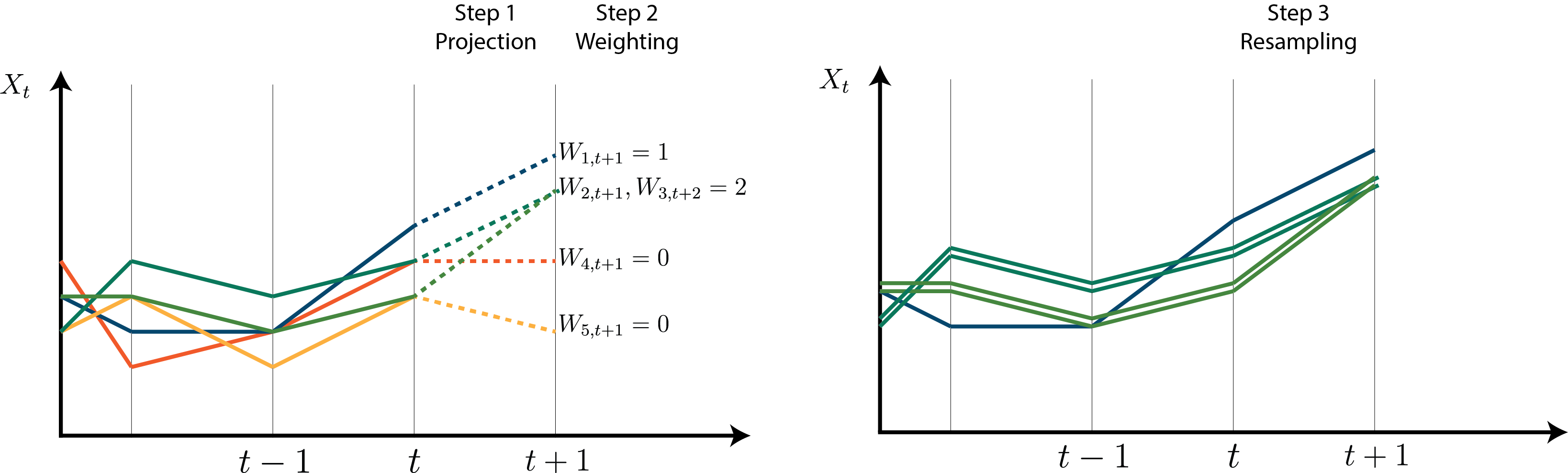
The bootstrap filter repeats three steps for each time step.
Assume we are at time step \(t\) and have a collection of samples from the filtering distribution at time \(t\!-\!1\), denoted \(\{x_{t-1}^{(i)}\}\), representing our guesses of the value of \(X_{t-1}\). We update these samples to represent our guesses of the value of \(X_t\) by:
Projecting them forward according to the state-space transition distribution.
Weighting these projected particles according to the observation distribution.
Resampling these particles according to their weights.
Figure 4.1: Diagram showing the three steps performed by the bootstrap filter at each time step \(t\). In this diagram, particle histories are also resampled, making this an example of a bootstrap smoother.
Step one creates a set of particles representing equally-likely one-step-ahead projections of \(X_t\) given data up to time \(t-1\):
And the final step resamples according to these weights to ensure the resulting \(\{x_t^{(i)}\}\) are equally-likely samples from \(P(X_t|y_{1:t}, \theta)\).
4.1.2 Simulation-based inference
In order to use SMC methods to fit a hidden-state model, we only need to:
Sample from the state-space transition distribution
Evaluate the observation distribution
Crucially, we do not need to evaluate the state-space transition distribution, allowing for easy simulation-based inference.
Simulation-based inference methods rely on simulations rather than analytical solutions and are very popular in statistical epidemiology. In this case, sampling from the state-space transition distribtion is the same as running the “simulator” one-step forward into the future. This simulator implies a likelihood even though we never need to find its precise form.
4.2 The bootstrap filter
Like before, assume that we have a collection of samples from the filtering distribution at time \(t\!-\!1\), denoted \(\{x_{t-1}^{(i)}\} \sim P(X_{t-1}|y_{1:t-1}, \theta)\). For now, also assume that our state-space transitions are Markovian (i.e., \(X_t\) depends only on \(X_{t-1}\)).
Step 1: Projection
By coupling these particles with the state-space transition model (Equation 3.1), we can make one-step-ahead predictions. Mathematically we want to obtain the predictive distribution: \[
\underbrace{P(X_t | y_{1:t-1}, \theta)}_{\text{predictive dist.}} = \int \underbrace{P(X_t | X_{t-1}, \theta)}_{\text{state-space transition dist.}} \underbrace{P(X_{t-1}|y_{1:t-1}, \theta)}_{\text{prev. filtering dist.}} \ dX_{t-1}
\]
Which is represented by complicated and potentially high-dimensional integral of two things we know. Fortunately, all we need to do is sample from the state-space transition model while conditioning on our particles:
Since we already have samples from the predictive distribution \(P(X_t | y_{1:t-1}, \theta)\), all we need to do is assign them weights \(w_t^{(i)}\) according to the observation distribution:
The final set of particles \(\{x_t^{(i)}\}\) is constructed by sampling (with replacement) from \(\{\tilde{x}_t^{(i)}\}\) according to the corresponding weights, resulting in:
\[
x_t^{(i)} \sim P(X_t | y_{1:t}, \theta)
\]
Repeat
Starting with an initial set of particles \(\{x_0^{(i)}\} \sim P(X_0)\), all we need to do is repeat this procedue for each \(t = 1, 2, \ldots, T\), storing the particle values as we go. This concludes the bootstrap filter.
The bootstrap filter is a special case of a sequential importance sampling algorithm (Section 4.6).
4.3 Fixed-lag smoothing
There are two problems with the bootstrap filter above:
It assumes the state-space transition model is Markovian (\(X_t\) depends only on \(X_{t-1}\))
\(X_t\) is informed by past data \(y_{1:t}\) only (the filtering posterior), when we may want to leverage all available data (the smoothing posterior).
Both of these problems are solved using fixed-lag resampling.
4.4 Algorithm
We present the algorithm as a Julia code-snippet. For a pseudocode implementation, please see our preprint.
The entire algorithm can be written in seven lines of code, although we use eight and some comments below for clarity. To fit a specific model, simply replace the initial distribution pX0, the state-space transition distribution pXt, and observation distribution pYt, with those of the hidden-state model.
# Inputs:# - θ: a parameter vector# - y: a vector of data# - N: the number of particles# - L: fixed-lag resampling window lengthfunctionSimpleBootstrapFilter(θ, y, N, L)# Pre-allocate an empty matrix of particles X =zeros(N, length(Ct))# Sample initial values X[:,1] =rand(pX0, N) # For each time step:for tt =2:length(Ct)# Project the hidden states X[:,tt] =rand.(pXt(X[:,tt-1], θ))# Calculate weights W =pdf.(pYt(X[:,tt], θ), y[tt])# Resample indices =wsample(1:N, W, N) X[:, max(tt-L, 1):tt] = X[indices, max(tt-L, 1):tt]endreturn(R, Y)end
4.5 Example
For demonstration, we consider a simple reproduction number estimator. First assume that \(\log R_t\) follows a Gaussian random walk with standard deviation \(0.2\):
Finally, we use a \(\text{Uniform}(0, 10)\) initial distribution for \(R_t\). This behaves somewhat like a prior distribution, except that resmapling ensures the early estimates of \(R_t\) reflect later data, so this has limited impact on the final estimates.
We load the same data used in the first two example models of the preprint. The entire algorithm (implemented below) takes approximately 0.4s to run on an M1 MacBook Pro.
usingStatsBase, Distributions, Plots, Measuresinclude("../src/LoadData.jl")functionrunSimpleExample()# Setup: N =10000# Number of particles T =100# Number of time steps ω =pdf.(Gamma(2.36, 2.74), 1:T) # Serial interval Y =loadData("NZCOVID") # Load data (Y is a DataFrame with column Ct) L =40# Fixed-lag resampling window# Pre-allocate and sample initial values: R =zeros(N, T) R[:,1] =log.(rand(Uniform(0, 10), N))# Run the bootstrap filter:for tt =2:T R[:,tt] =rand.(Normal.(R[:,tt-1], 0.2)) # Project Rt Λ =sum(Y.Ct[(tt-1):-1:1] .* ω[1:(tt-1)]) # Calculate the force-of-infection W =pdf.(Poisson.(Λ *exp.(R[:,tt])), Y.Ct[tt]) # Calculate weights R[1:N, max(tt-L, 1):tt] = R[wsample(1:N, W, N), max(tt-L, 1):tt] # Resampleend# Process and plot the results m =vec(mean(exp.(R), dims=1)) l = [quantile(Rt, 0.025) for Rt ineachcol(exp.(R))] u = [quantile(Rt, 0.975) for Rt ineachcol(exp.(R))]plot(Y.date, m, ribbon=(m-l, u-m), size=(800,400), xlabel="Date", ylabel="Reproduction number", label=false, margins=3mm)endrunSimpleExample()
Julia
The total elapsed time is \(<1\)s. If running this example locally, the first time may take longer as Julia must compile the function and load the plotting backend. This long “time-to-first-plot” is a well-known annoyance in Julia.
4.5.1 Choosing the number of particles
In the example above, we used \(N = 10{,}000\) particles. Heuristically, we can check whether \(N\) is large enough by refitting the model and checking that our results are visually stable.
Alternatively, the effective sample size (ESS) is a measure of the number of independent samples that would be equivalent to a given weighted sample (Elvira, Martino, and Robert 2022). It is typically written as:
where \(\bar{w}_i\) is the normalised weight of the \(i^{th}\) sample. As we resample past states without tracking particle weights we cannot directly apply this formula. Instead, we approximate it using:
where \(n_j\) is the number of times that the \(j^{th}\) unique value features in the resampled set of particles (and \(M\) is the total number of unique particles after resampling). We calculate this after running the bootstrap filter using:
functionapproximateESS(Rvec) N =length(Rvec)# Fetch a dictionary of the unique values of Rvec and the count nj =countmap(vec(Rvec)) # Compute ESS approximation ESS =1/sum([(v/N)^2 for v invalues(nj)])return(ESS)end
We apply this to each column of R in the example above to estimate the ESS (full code is collapsed for brevity):
ESS = [approximateESS(Rt) for Rt ineachcol(R)]
Code
usingStatsBase, Distributions, Plots, Measuresinclude("../src/LoadData.jl")functionrunSimpleExampleWithESS()# Setup: N =10000# Number of particles T =100# Number of time steps ω =pdf.(Gamma(2.36, 2.74), 1:T) # Serial interval Y =loadData("NZCOVID") # Load data (Y is a DataFrame with column Ct) L =40# Fixed-lag resampling window# Pre-allocate and sample initial values: R =zeros(N, T) R[:,1] =log.(rand(Uniform(0, 10), N))# Run the bootstrap filter:for tt =2:T R[:,tt] =rand.(Normal.(R[:,tt-1], 0.2)) # Project Rt Λ =sum(Y.Ct[(tt-1):-1:1] .* ω[1:(tt-1)]) # Calculate the force-of-infection W =pdf.(Poisson.(Λ *exp.(R[:,tt])), Y.Ct[tt]) # Calculate weights R[1:N, max(tt-L, 1):tt] = R[wsample(1:N, W, N), max(tt-L, 1):tt] # Resampleend# Process and plot the effective sample size ESS = [approximateESS(Rt) for Rt ineachcol(R)]plot(Y.date, ESS, size=(800,400), xlabel="Date", ylabel="Effective sample size", label=false, margins=3mm)endrunSimpleExampleWithESS()
The ESS decreases rapidly as we move left along the x-axis. In general we expect the ESS at all \(t < T - L\) to be similar (i.e. the plot of ESS against time should be flat until the final \(L\) time steps). In this example, the data are more unpredictable in earlier time-steps, which causes the projection step to select fewer “good” particles, thus also decreasing the ESS.
In this example, the minimum ESS is 36, which results in unstable credible intervals for estimates at small \(t\). The ESS can be increased by:
Increasing \(N\)
Decreasing \(L\)
Fitting a “better” model (one where the projections are more likely)
Using more complex tools from the SMC literature, such as an auxillary particle filter, which uses future data in the proposal density (Doucet and Johansen 2011)
In this case, increasing \(N\) to \(100{,}000\) only adds a couple of seconds of computation time, and results in much more stable estimates (a minimum ESS of approximately 360).
4.6 Additional resources
Bootstrap filters (and SMC methods more generally) have found use in many fields. Each field has their own motivation for and notation describing these methods. We provide an overview of other resources here.
Those with an engineering background may be familiar with “filtering and smoothing”, where the state of a time-varying system is tracked through the observation of noisy measurements. Classical examples include GPS position tracking or audio signal processing.
The Kalman filter, which provides an analytical solution when the state-space transition and observation models are linear Gaussian and Markovian, is perhaps the best-known example of a filtering method from engineering.
Chapters 7 and 11 of Särkkä (2013) introduce SMC methods under the headings “particle filtering” and “particle smoothing”. We also recommend chapters 1 (What are Bayesian filtering and smoothing?), 4 (Bayesian filtering equations and exact solutions), and 8 (Bayesian smoothing equations and exact solutions).
A survey of Sequential Monte Carlo Methods for Economics and Finance (Creal 2012)
Those with an econometrics background may find this extensive review helpful, although the author focusses on Markovian models. Examples employed in this review include a stochastic volatility model and a nonlinear dynamic stochastic general equilibrium model.
Those with a background in atmospheric science, oceanography, meteorology, or other environmental sciences may be familiar with “data assimilation”, where focus is placed on combining model predictions with observational data. Chapter 9 of this book introduces particle filters as a method for solving the “fully nonlinear data assimilation” problem.
This list is incomplete. If you know of any additional resources that may be helpful, please get in touch!
Doucet, Arnaud, and Adam M. Johansen. 2011. “A Tutorial on Particle Filtering and Smoothing : Fiteen Years Later.” In, edited by Dan Crisan and Boris Rozovskii, 656–705. Oxford ; N.Y.: Oxford University Press.
Elvira, Víctor, Luca Martino, and Christian P. Robert. 2022. “Rethinking the Effective Sample Size.”International Statistical Review 90 (3): 525–50. https://doi.org/10.1111/insr.12500.
Evensen, Geir, Femke C. Vossepoel, and Peter Jan Van Leeuwen. 2022. Data Assimilation Fundamentals: A Unified Formulation of the State and Parameter Estimation Problem. Springer Textbooks in Earth Sciences, Geography and Environment. Cham: Springer International Publishing. https://doi.org/10.1007/978-3-030-96709-3.